
Table of Contents
The Morphogenesis of Tree Bark in Algorithmic Space
When we look at nature, our eyes recognize living patterns instantly. Biophilic design teaches us that humans have an innate need to connect with natural systems. In digital spaces, bringing nature to life is more than just pasting a static photo onto a screen. Standard photographic textures repeat across large surfaces, and the human brain quickly spots those artificial tiles. That repetition causes visual fatigue and breaks the feeling of immersion.
To build a convincing digital world, we must create surfaces that grow, shift, and show natural irregularity. Learning how to create an authentic organic bark texture using code gives you complete creative control. Instead of relying on heavy image files that slow down web pages, we can calculate surface details mathematically directly on the graphics card.
The main problem in computer graphics is that pure mathematical noise often looks artificial. If you sample standard Perlin noise on a cylinder, you do not get the rough, weathered appearance of a forest tree. Instead, you get something that looks like smooth, melted plastic or polished marble. Natural tree bark forms through intense physical stress. Living wood inside a tree expands outward each year, splitting the dead outer layer into ragged ridges, deep cracks, and rough plates. A single mathematical function cannot capture those competing biological forces.
To solve this, we use a procedural pipeline written in GLSL (OpenGL Shading Language). By combining anisotropic UV coordinates, cellular noise, and layered domain warping, we can simulate physical growth and stress fractures on the GPU. This procedural pipeline builds an authentic organic bark texture from raw math. It produces zero network download overhead, provides infinite resolution, and captures the tactile quality of the forest canopy right in the browser.
The Biophilic Imperative in Modern Web Design
Biophilic web design brings natural forms, textures, and rhythms into digital interfaces. For decades, digital design focused on flat surfaces, hard rectangles, and artificial gradients. While those styles work well for basic data entry, they feel cold and disconnected from human biology. Natural environments are rich in organized complexity. In nature, patterns repeat across different scales without ever being completely identical.
Scientific studies show that viewing natural fractal patterns reduces stress levels in the human body. Fractal patterns with a dimension between 1.3 and 1.5 help human eyes relax because our visual system evolved to process natural scenery like clouds, forest canopies, and rough coastlines. When you use an organic bark texture in a web environment, you tap into that deep visual comfort.
A procedural organic bark texture brings warmth and physical grounding to a digital layout. Rather than distracting the visitor, procedural nature patterns create a calming backdrop that keeps visitors engaged longer. By building dynamic materials directly into the rendering pipeline, we turn cold browser windows into living, restorative spaces.
The Basic Problem: Why Simple Noise Looks Like Plastic
Most developers who try to write a procedural shader start by downloading a basic 2D noise script. They plug their UV coordinates into the noise function, multiply it by brown paint, and wonder why the surface looks artificial. Standard noise algorithms like Perlin or Simplex noise distribute energy evenly across all directions. They produce soft, rounded mounds that resemble smooth clay or clouds.
Real tree bark never grows in soft, symmetrical mounds. Tree growth is directional. As a trunk grows taller and thicker, vertical fibers stretch while outward pressure tears the surface apart. A convincing organic bark texture requires sharp directional contrasts, ragged plateaus, and dark, recessed fissures.
When you apply isotropic noise to a 3D tree trunk, the surface looks synthetic. It lacks the sharp structural breaks and vertical grain that tell the human eye they are looking at real wood. To solve this fundamental problem, we must study the actual biology of trees and translate those physical growth rules into our shader calculations.
Overview of the Procedural Pipeline
Our procedural pipeline runs inside a fragment shader, executing code for every pixel simultaneously. We begin by taking the surface coordinates of our 3D model and stretching them along the vertical axis. This directional stretching mimics the vertical orientation of wood fibers.
Next, we calculate the primary fissures using cellular noise, also known as Worley noise. This step breaks the surface into discrete, interlocking bark plates. We then distort those coordinates using a technique called domain warping. Domain warping feeds one layer of noise into the inputs of another layer, bending straight lines into twisted, organic paths.
After shaping the large cracks, we add multiple octaves of high-frequency noise to build tiny ridges and rough surface fibers. Once this combined heightfield is complete, we calculate surface lighting normals using finite differences. Finally, we map those geometric heights into a natural color palette. The entire pipeline turns pure math into a rich organic bark texture running at sixty frames per second.
+--------------------------------------------------------+
|              Normalized UV Coordinates                 |
+--------------------------------------------------------+
                           |
                           v
+--------------------------------------------------------+
|      Anisotropic Scaling (Vertical Fiber Stretch)      |
+--------------------------------------------------------+
                           |
                           v
+--------------------------------------------------------+
|    Domain Warping (Coordinates Perturbed by Noise)     |
+--------------------------------------------------------+
                           |
                           v
+--------------------------------------------------------+
|      Multi-Octave fBm + Worley Cellular Cracks         |
+--------------------------------------------------------+
                           |
                           v
+--------------------------------------------------------+
|       Synthesized Heightfield & Crevice Mask           |
+--------------------------------------------------------+
              |                             |
              v                             v
+---------------------------+ +--------------------------+
| Finite-Difference Normals | | Dynamic Color & PBR Maps |
+---------------------------+ +--------------------------+
              \                             /
               \                           /
                v                         v
+--------------------------------------------------------+
|         Final Shaded Organic Bark Surface              |
+--------------------------------------------------------+
Biological Foundations: Deconstructing the Anatomy of Rhytidome
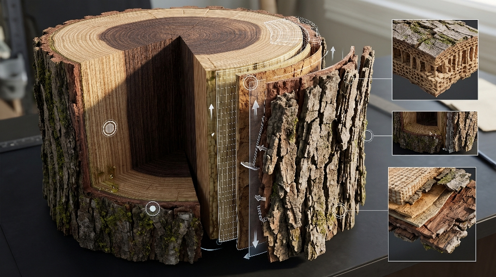
To write believable graphics code, you must first understand the physical material you are modeling. In botany, the rough outer layer that we call bark is technically named the rhytidome. The rhytidome is a protective barrier of dead cells that shields the living inner tree from drought, insects, fungi, and fire.
By studying how the rhytidome forms, we can write shader math that simulates real biological processes. An authentic organic bark texture should look like it grew over decades through cycles of seasonal expansion and weather exposure.
       [ Cross-Section of a Mature Tree Trunk ]

                 (+++++)  <-- Outer Bark (Rhytidome / Fissures)
                ( +++++ )
               (  =====  ) <-- Cork Cambium (Phellogen)
              (   .....   ) <-- Living Phloem (Inner Bark)
             (    *****    ) <-- Vascular Cambium (Growth Layer)
            (     #####     )
           (      #####      ) <-- Sapwood (Active Xylem)
          (       #####       )
         (        @@@@@        ) <-- Heartwood (Dense Structural Core)
Botanical Growth Mechanics
A tree grows thicker from an internal ring of active cells called the vascular cambium. Each spring and summer, this layer produces new wood cells on the inside and new food-transporting cells on the outside. Because the tree produces new tissue underneath an already hardened exterior, the outer circumference must either stretch or burst.
The dead outer cells cannot stretch very far. As the inner trunk expands, it creates intense mechanical tension known as circumferential hoop stress. When this stress exceeds the strength of the outer bark cells, the outer layer fractures.
These tears run predominantly parallel to the trunk because the internal wood cells grow in vertical columns. As the tree continues to age, new layers of cork cambium form beneath the fissures, pushing older, dead layers outward. This continuous cycle of internal pushing and external cracking gives an organic bark texture its deep, ragged relief.
Morphological Classification of Bark Surfaces
Different tree species solve growth stress in distinct ways, producing unique surface structures:
- Longitudinal Fissures: Seen on mature oaks, chestnuts, and pines. The bark breaks into deep vertical trenches separated by hard, flat ridges.
- Exfoliating Papery Sheets: Seen on birch trees. The outer layer separates along horizontal lines, peeling away in thin, flexible ribbons.
- Scaly Mosaic Plates: Seen on sycamore, spruce, and mature pines. The bark fractures along both vertical and horizontal lines, creating overlapping scales that flake off over time.
- Smooth Lenticellate Surfaces: Seen on young cherry trees. The bark remains mostly smooth, marked only by small, horizontal breathing pores called lenticels.
For our procedural shader, we will focus on longitudinal fissuring. This structure produces dramatic depth, casts rich shadows, and showcases the full power of procedural coordinate distortion.
Translating Biology into Vector Math
To turn these biological growth rules into vector math, we must break down the physical forces into coordinate operations. First, wood grain runs vertically, so we scale our coordinate system unevenly. If we multiply the horizontal coordinate by a large number and the vertical coordinate by a small number, our noise stretches out into tall, thin bands.
Second, the cracks between bark plates are not straight cuts. As the bark pulls apart, it twists around knots, old branch locations, and irregular grain lines. We can model this wandering path by shifting our coordinate grid using smooth noise functions before calculating our cracks.
Finally, older bark ridges weather away from wind and rain, rounding their sharp edges, while fresh cracks expose steep, rough valleys. In our shader math, we can create steep, flat-topped ridges by running our noise outputs through non-linear curves like power functions and smooth minimums. This gives our organic bark texture the authentic look of hard, weathered wood.
Noise Primitives: Why Single Noise Algorithms Fail
Every procedural shader depends on noise primitives as its raw building blocks. A noise primitive is simply a mathematical function that takes a coordinate as input and returns a pseudo-random value between zero and one. However, using just one type of noise will never produce a convincing organic bark texture. Let us examine the main noise types and see how each contributes to the final result.
| Noise Primitive Type | Computational Cost | Visual Pattern Shape | Primary Structural Function in Bark |
| Value Noise | Very Low | Blocky, linear gradients | Secondary coordinate perturbation |
| Perlin Noise | Low | Soft, directional grid bands | Broad underlying surface swell |
| Simplex Noise | Moderate | Smooth, omnidirectional waves | Fine fibrous micro-creases |
| Worley / Cellular (F1) | High | Sharp polygonal cells | Raised bark plates and shields |
| Worley Edge (F2 – F1) | High | Deep, narrow webbed fissures | Primary growth stress cracks |
Simplex vs. Perlin vs. Value Noise
Value noise is the simplest form of noise. It assigns random values to a grid of points and interpolates smoothly between them. While it runs very fast on low-power devices, it often shows visible grid patterns. It looks too blocky to serve as the main surface for an organic bark texture.
Perlin noise improves on value noise by assigning random gradient vectors to grid corners instead of simple values. This creates organic hills and valleys. However, classic Perlin noise still aligns with a square grid, which can cause subtle horizontal and vertical artifacts.
Simplex noise solves these directional flaws by dividing space into triangles rather than squares. Simplex noise produces smooth, continuous waves without visible grid alignment. It is ideal for rendering fine, fibrous micro-details and soft underlying undulations across our organic bark texture.
Cellular (Worley/Voronoi) Noise
Cellular noise, introduced by Steven Worley, works differently from gradient noise. Instead of using a grid of smooth hills, it scatters random feature points throughout space. For any given coordinate, the function finds the distance to the closest feature point. This calculation produces a network of convex cells that looks like biological tissue, dried mud, or reptile scales.
+-------------------------------------------------------+
|  Cellular Noise Logic: Distance to Feature Points     |
|                                                       |
|        * P1                                           |
|         \                                             |
|          \  d1 (Shortest distance = F1)               |
|           \                                           |
|            x (Current Fragment UV)                    |
|             \                                         |
|              \  d2 (Second shortest = F2)             |
|               \                                       |
|                * P2                                   |
|                                                       |
|   Crack Value = F2 - F1  (Smallest along boundaries)  |
+-------------------------------------------------------+
By calculating both the distance to the nearest point (F1) and the distance to the second-nearest point (F2), we can subtract F1 from F2. Along the boundaries between cells, those two distances are nearly identical, which means F2 – F1 drops down to zero.
This simple subtraction creates a sharp network of dark boundary lines. These narrow boundary lines perfectly match the deep cracks that separate individual bark plates on an old tree. Cellular noise gives our organic bark texture structural cracks that gradient noise cannot create on its own.
Fractional Brownian Motion (fBm)
A single layer of noise looks flat and uniform because it only has one level of scale. Real natural structures exhibit self-similarity, meaning they reveal smaller and smaller versions of the same patterns as you look closer. We reproduce this self-similar detail using Fractional Brownian Motion, commonly abbreviated as fBm.
In an fBm loop, we sample a noise function multiple times, with each pass called an octave. With every new octave, we double the frequency so the pattern repeats twice as fast. At the same time, we cut the amplitude in half so the smaller details do not overwhelm the larger forms.
By adding six or seven octaves together, we create a complex heightfield with big rolling hills, medium-sized ledges, and tiny sand-like bumps. Using fBm is essential for turning flat geometry into an authentic, touchable organic bark texture.
Mathematical Architecture: Implementing Anisotropic Domain Warping
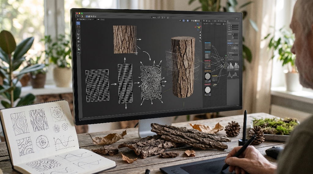
Now that we have our basic noise tools, we need to arrange them into an artistic structure. If you simply layer noise on a standard surface, you will end up with an unorganized collection of bumps. To create the look of genuine tree bark, we use two advanced mathematical techniques: anisotropic coordinate transformation and domain warping.
       [ Step-by-Step Coordinate Distortion ]

 (1) Standard UV Grid       (2) Anisotropic Stretch     (3) Domain Warped Grid
   +---+---+---+              +-------+-------+           + ~ ~ + ~ ~ +
   |   |   |   |              |       |       |           |  ~    ~   |
   +---+---+---+    ===>      +-------+-------+   ===>    +  ~   ~  ~ +
   |   |   |   |              |       |       |           | ~   ~   ~ |
   +---+---+---+              +-------+-------+           + ~ ~ + ~ ~ +
  (Equal X and Y)             (Stretched X >> Y)          (Turbulent Flow)
Coordinate Space Transformations
Anisotropy means having properties that differ depending on the direction you measure. Since trees grow vertically toward the sun, tree bark has strong directional bias. Wood fibers are tall, thin, and closely packed side by side.
We begin our fragment shader by modifying the incoming texture coordinates. If our input coordinates are represented by a two-dimensional vector called uv, we can multiply the horizontal coordinate by a large factor while scaling the vertical coordinate down:
OpenGL Shading Language
vec2 barkUV = vec2(uv.x * 4.0, uv.y * 0.8);
This single line of code stretches our coordinate space horizontally across the screen. Any circular noise shape placed into this space automatically becomes an elongated vertical oval. This sets up the natural vertical orientation needed for a lifelike organic bark texture.
The Principle of Domain Warping
Domain warping is one of the most powerful tools in procedural graphics. In a standard shader, you pass your clean coordinates directly into a noise function to read a height value. In domain warping, you use one noise function to distort the coordinates before feeding them into a second noise function.
Think of it like drawing a neat checkerboard on a sheet of soft rubber. If you stretch and twist the rubber sheet with your hands, the straight lines bend into swirling curves. In code, we calculate a vector offset using two noise functions, scale that offset by a chosen strength, and add it directly to our position coordinates:
pdistorted = p + α X noise(p)
We can even repeat this process by feeding the warped coordinates into a third noise function. This multi-stage distortion creates flowing, liquid-like trails that look remarkably like natural wood grain. Domain warping transforms rigid, mechanical patterns into a dynamic, living organic bark texture.
Directional Furrow Shaping
If we apply domain warping equally in all directions, our bark will swirl around like marble cake. To keep the look of wood, our coordinate distortion must follow the direction of the trunk.
We achieve this by giving our warping vectors their own directional bias. We allow the coordinates to shift strongly from side to side across the horizontal axis, but keep vertical movement minimal. This mimics the way expanding wood fibers separate laterally while remaining anchored vertically.
By steering the distortion along the growth axis, our cracks wander naturally around invisible barriers without ever losing their vertical rhythm. This disciplined distortion ensures our organic bark texture looks structurally solid and botanically accurate.
Step-by-Step GLSL Implementation: The Fragment Pipeline
Let us look at the practical code needed to run this procedural pipeline. We will write a complete fragment shader that you can load directly into a WebGL context, a Three.js material, or an online shader tool.
       [ Shader Fragment Pipeline Assembly ]

   varying vec2 vUv ───► [ Anisotropic Stretch ]
                                │
                                ▼
                         [ Domain Warp ]
                         /             \
                        v               v
                [ Worley Noise ]   [ Simplex fBm ]
                 (Major Cracks)    (Surface Roughness)
                        \               /
                         v             v
                    [ Non-Linear Ridge Shaper ]
                                │
                                ▼
                    [ Final Height Output ]
                                │
                                ▼
                    [ Finite-Diff Normal Map ]
Boilerplate and Uniform Setup
We start by declaring our precision settings and receiving the standard uniforms from the rendering engine. We need the current screen resolution, a time uniform for optional wind or growth movement, and our varying UV coordinates passed from the vertex stage:
OpenGL Shading Language
precision highp float;

uniform vec2 u_resolution;
uniform float u_time;
varying vec2 vUv;

#define PI 3.14159265359
Using high precision is essential for procedural noise. Medium precision can cause visible banding artifacts and precision loss on mobile graphics chips when performing deep mathematical loops.
Constructing the Custom Noise Library in GLSL
Next, we need an efficient noise function that runs without external image textures. Here is a fast, permutation-free 2D gradient noise implementation, followed by a cellular Worley function:
OpenGL Shading Language
// Hash function for pseudo-random 2D vectors
vec2 hash2(vec2 p) {
    p = vec2(dot(p, vec2(127.1, 311.7)),
             dot(p, vec2(269.5, 183.3)));
    return -1.0 + 2.0 * fract(sin(p) * 43758.5453123);
}

// 2D Gradient Noise
float gradientNoise(vec2 p) {
    vec2 i = floor(p);
    vec2 f = fract(p);
    vec2 u = f * f * (3.0 - 2.0 * f);

    return mix(mix(dot(hash2(i + vec2(0.0, 0.0)), f - vec2(0.0, 0.0)),
                   dot(hash2(i + vec2(1.0, 0.0)), f - vec2(1.0, 0.0)), u.x),
               mix(dot(hash2(i + vec2(0.0, 1.0)), f - vec2(0.0, 1.0)),
                   dot(hash2(i + vec2(1.0, 1.0)), f - vec2(1.0, 1.0)), u.x), u.y);
}

// Worley Cellular Noise returning F1 and F2
vec2 cellularNoise(vec2 p) {
    vec2 n = floor(p);
    vec2 f = fract(p);
    float f1 = 8.0;
    float f2 = 8.0;

    for (int j = -1; j <= 1; j++) {
        for (int i = -1; i <= 1; i++) {
            vec2 g = vec2(float(i), float(j));
            vec2 o = hash2(n + g) * 0.5 + 0.5;
            vec2 delta = g + o - f;
            float d = dot(delta, delta);

            if (d < f1) {
                f2 = f1;
                f1 = d;
            } else if (d < f2) {
                f2 = d;
            }
        }
    }
    return vec2(sqrt(f1), sqrt(f2));
}
These two functions serve as our foundation. The gradient noise produces smooth background undulations, while the cellular noise calculates the sharp plateaus and valleys that give an organic bark texture its signature look.
Assembling the Multi-Scale Bark Heightmap
Now we combine these primitives into our complete height function. We will build an fBm loop to create our domain warp, apply anisotropic scaling, and combine the results into a single heightfield value:
OpenGL Shading Language
// Fractional Brownian Motion for surface grain
float fbm(vec2 p) {
    float total = 0.0;
    float amplitude = 0.5;
    mat2 rot = mat2(cos(0.5), sin(0.5), -sin(0.5), cos(0.5));

    for (int i = 0; i < 5; i++) {
        total += amplitude * gradientNoise(p);
        p = rot * p * 2.02;
        amplitude *= 0.5;
    }
    return total;
}

// Master height function representing the bark surface
float calculateBarkHeight(vec2 uv) {
    // 1. Anisotropic coordinate stretch
    vec2 p = vec2(uv.x * 6.0, uv.y * 1.5);

    // 2. Domain warping vectors
    vec2 warpA = vec2(fbm(p + vec2(0.0, 0.0)), fbm(p + vec2(5.2, 1.3)));
    vec2 warpB = vec2(fbm(p + warpA * 1.5 + vec2(1.7, 9.2)),
                      fbm(p + warpA * 1.5 + vec2(8.3, 2.8)));

    vec2 warpedPos = p + warpB * 0.8;

    // 3. Primary structural cracks via Worley cellular boundaries
    vec2 cell = cellularNoise(warpedPos * 1.2);
    float crackPattern = cell.y - cell.x; // F2 - F1 generates boundary borders
    crackPattern = smoothstep(0.05, 0.35, crackPattern);

    // 4. Fine surface grain fibers
    float microGrain = fbm(warpedPos * 4.0) * 0.35;

    // 5. Combine layers into unified heightfield
    float finalHeight = crackPattern * 0.7 + microGrain * 0.3;
    return clamp(finalHeight, 0.0, 1.0);
}
This master function calculates the complete structure of our organic bark texture. Every coordinate now maps to a precise physical height that captures both broad tree plates and delicate surface fibers.
Carving Deep Cavities
In real wood, cracks are not smooth parabolic valleys. They are deep, shadowed ravines where light struggles to enter. To simulate these dark crevasses, we sharpen our height transitions using mathematical power curves.
By running our raw crack value through a non-linear pow function or a steep smoothstep, we push the bottom of the fissures down toward zero while keeping the tops of the bark plates relatively flat. This mimics how the tough outer bark resists erosion while the cracks between plates pull open. This step gives an organic bark texture its striking depth and dramatic appearance.
Deriving Surface Normals and Tangent-Space Lighting
A heightmap alone cannot react to light. To make our procedural surface look three-dimensional, we must compute surface normal vectors. A normal vector is an arrow pointing straight out from the surface, showing which way that pixel faces.
In traditional game development, artists pre-render normal vectors into RGB image files called normal maps. Because our organic bark texture lives entirely inside code, we calculate these normal vectors on the fly for every frame.
          [ Finite Difference Normal Calculation ]

                           H(uv + (0, e))
                                 |
                                 |
        H(uv - (e, 0)) ──── Fragment UV ──── H(uv + (e, 0))
                                 |
                                 |
                           H(uv - (0, e))

     Normal Vector = normalize( vec3( dH/dx, 2.0 * epsilon, dH/dy ) )
Analytic vs. Numerical Normals on the GPU
There are two ways to derive surface normals from a procedural math function: analytic derivation and numerical calculation. Analytic derivation involves writing out the exact calculus derivative of our noise equations. While mathematically pure, calculating the exact derivative of multiple nested, domain-warped noise functions requires massive amounts of code and quickly overwhelms the GPU.
Numerical calculation, known as finite differences, is much more practical. Instead of solving complex calculus equations, we sample our height function a few times at tiny offsets to see how quickly the height changes. This slope measurement tells us which way the surface tilts, allowing us to build an accurate normal vector with minimal code.
Calculating Normals via Finite Differences
To calculate finite differences on the GPU, we pick a tiny offset distance called epsilon. We sample our height function slightly to the left, slightly to the right, slightly above, and slightly below our current pixel:
OpenGL Shading Language
vec3 calculateBarkNormal(vec2 uv, float strength) {
    vec2 eps = vec2(0.005, 0.0);

    float hL = calculateBarkHeight(uv - eps.xy);
    float hR = calculateBarkHeight(uv + eps.xy);
    float hD = calculateBarkHeight(uv - eps.yx);
    float hU = calculateBarkHeight(uv + eps.yx);

    // Calculate slopes along X and Y axes
    float dX = (hR - hL);
    float dY = (hU - hD);

    // Construct the 3D normal vector
    vec3 normal = normalize(vec3(-dX * strength, 2.0 * eps.x, -dY * strength));
    return normal;
}
This function returns a normalized three-dimensional vector. When light hits a ridge facing the light source, the surface brightens. When light grazes a steep crevice, the surface turns dark. This real-time lighting response makes our organic bark texture pop off the screen with rich three-dimensional relief.
Hardware Derivatives Alternative
GLSL provides another way to compute slopes using built-in hardware derivative functions: dFdx() and dFdy(). The graphics hardware evaluates four adjacent pixels simultaneously in two-by-two screen blocks. Because it already knows the values at neighboring pixels, it can estimate the surface slope without running the height function extra times.
While hardware derivatives run extremely fast, they can introduce a subtle stepping effect on steep procedural ridges. For high-end desktop screens, the four-tap finite difference method produces a much cleaner organic bark texture. On lower-end mobile devices, switching to hardware derivatives can save battery power and maintain high frame rates.
Ambient Occlusion and Cavity Darkening
In real life, light bounces off surrounding surfaces. Open plains receive light from the entire sky, but the bottom of a narrow bark crack receives almost no bounced light. This natural darkening effect is called ambient occlusion.
We can approximate ambient occlusion directly from our procedural height value. Because our cracks are the lowest points in the heightfield, low height values naturally receive less ambient light:
OpenGL Shading Language
float ambientOcclusion = smoothstep(0.0, 0.6, barkHeight);
Multiplying our final lighting calculations by this simple cavity factor darkens the deep fissures, giving our organic bark texture rich contrast and depth.
Naturalistic Color Palettes and Physical Material Mapping
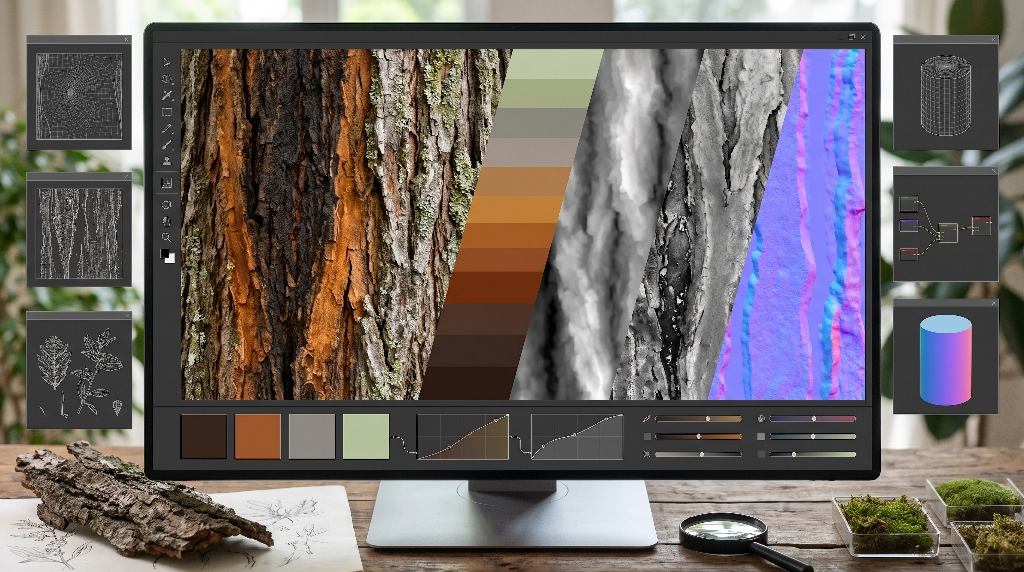
A common mistake in digital design is making tree bark a flat, uniform brown. In natural forests, tree bark contains a surprising variety of rich, layered colors.
Healthy bark surfaces are covered with life and weathering effects, including dead tannins, green moss, dusty grey lichens, and exposed inner wood. To build a lifelike organic bark texture, our shader must paint across this rich natural spectrum.
             [ Color Mapping by Surface Elevation ]

  Elevation Height    Color Tone              Botanical Context
  ---------------------------------------------------------------------
  1.0 (Ridge Top)     Light Silver-Grey       Weathered Lichen Colonies
  0.7 (Plate Face)    Desaturated Raw Umber   Oxidized Cork Layer
  0.4 (Flank Slope)   Warm Sienna / Amber     Freshly Exposed Cambium
  0.0 (Crevice Floor) Near-Black Burnt Brown  Damp, Shaded Cavities
Beyond Monochromatic Brown
Natural pigments break down into distinct botanical layers. The outer cells contain dark tannins and suberin, a waxy compound that seals moisture inside the tree. These dead tissues weather under sun and rain, turning a silvery grey or cool charcoal.
When wind or animal friction breaks an outer plate, the fresh cork beneath shows warmer amber and golden-brown tones. Inside deep cracks, accumulated moisture supports colonies of microscopic algae and fungi, creating subtle olive-green stains. Incorporating these varied pigments ensures your organic bark texture looks like living forest growth rather than molded plastic.
Multi-Stop Color Ramps in GLSL
We can implement this natural color variety in GLSL by building a multi-stop color ramp that samples colors based on surface height and slope steepness:
OpenGL Shading Language
vec3 getBarkColor(float height, vec3 normal, vec2 uv) {
    // 1. Define botanical color swatches
    vec3 creviceColor = vec3(0.08, 0.05, 0.03);  // Deep burnt umber
    vec3 flankColor   = vec3(0.28, 0.17, 0.10);  // Warm raw sienna
    vec3 ridgeColor   = vec3(0.42, 0.35, 0.28);  // Weathered grey-brown
    vec3 lichenColor  = vec3(0.45, 0.48, 0.38);  // Pale olive-grey lichen

    // 2. Interpolate base tones across the heightfield
    vec3 baseColor = mix(creviceColor, flankColor, smoothstep(0.0, 0.4, height));
    baseColor = mix(baseColor, ridgeColor, smoothstep(0.4, 0.85, height));

    // 3. Add lichen patches on upward-facing high plateaus
    float lichenMask = smoothstep(0.7, 0.9, height) *
                       smoothstep(0.2, 0.6, gradientNoise(uv * 12.0));
    vec3 finalColor = mix(baseColor, lichenColor, lichenMask * 0.6);

    return finalColor;
}
This function creates a rich, layered material. The deep cracks stay dark and shaded, the ridge flanks display warm wood tones, and the high ridges show cool, weathered highlights. This color balance gives the organic bark texture an authentic forest appearance.
Synthesizing PBR Outputs
Modern 3D web engines rely on Physically Based Rendering, commonly called PBR. PBR materials use several paired maps to control how light interacts with a surface: Albedo (base color), Roughness (surface polish), and Metallic properties.
OpenGL Shading Language
// Invert height to generate realistic roughness
// Crevices retain dampness (lower roughness); ridges are dry and powdery (matte)
float roughnessMap = mix(0.45, 0.95, height);

// Wood has zero metallic reflectance
float metallicMap = 0.0;
Dry outer bark is an excellent light diffuser, with a high roughness value between 0.85 and 0.95. However, inside deep, damp fissures, the roughness drops toward 0.45, giving those shaded cracks a slight sheen as if holding moisture. Generating these PBR values in code makes our organic bark texture respond realistically under dynamic environment maps and moving scene lights.
WebGL and Three.js Production Integration
Now that our shader code is written, we need to integrate it into a real production environment. Three.js is the most popular 3D library for web browsers, providing an easy-to-use bridge between modern JavaScript and low-level WebGL graphics hardware.
       [ Production Three.js Architecture ]

   +-------------------------------------------------------+
   |                Three.js Scene Graph                   |
   |                                                       |
   |   [ PerspectiveCamera ]       [ DirectionalLight ]    |
   |             \                         /               |
   |              \                       /                |
   |               v                     v                 |
   |           +-------------------------------+           |
   |           |          Mesh Object          |           |
   |           |  Geometry: Cylinder / Trunk   |           |
   |           |  Material: ShaderMaterial     |           |
   |           +---------------+---------------+           |
   +---------------------------|---------------------------+
                               v
   +-------------------------------------------------------+
   |             WebGL GPU Fragment Processing             |
   |                                                       |
   |   - Unrolled Math Loops                               |
   |   - Dynamic Resolution Uniforms                       |
   |   - Continuous Real-Time Evaluation                   |
   +-------------------------------------------------------+
Custom ShaderMaterial Setup
To run our procedural GLSL code inside Three.js, we wrap it in a ShaderMaterial. This class lets us feed custom uniforms, vertex transformations, and fragment shaders directly to the graphics card:
JavaScript
import * as THREE from 'three';

const barkMaterial = new THREE.ShaderMaterial({
  uniforms: {
    u_time: { value: 0.0 },
    u_resolution: { value: new THREE.Vector2(window.innerWidth, window.innerHeight) },
    u_lightPos: { value: new THREE.Vector3(5.0, 10.0, 7.0) }
  },
  vertexShader: `
    varying vec2 vUv;
    varying vec3 vNormal;
    varying vec3 vWorldPosition;

    void main() {
      vUv = uv;
      vNormal = normalize(normalMatrix * normal);
      vec4 worldPos = modelMatrix * vec4(position, 1.0);
      vWorldPosition = worldPos.xyz;
      gl_Position = projectionMatrix * viewMatrix * worldPos;
    }
  `,
  fragmentShader: `
    // Insert all our custom GLSL functions here
    // calculateBarkHeight, calculateBarkNormal, getBarkColor...

    varying vec2 vUv;
    varying vec3 vNormal;
    varying vec3 vWorldPosition;
    uniform vec3 u_lightPos;

    void main() {
      float h = calculateBarkHeight(vUv);
      vec3 normal = calculateBarkNormal(vUv, 2.5);
      vec3 albedo = getBarkColor(h, normal, vUv);

      // Simple Lambertian Diffuse Lighting
      vec3 lightDir = normalize(u_lightPos - vWorldPosition);
      float diff = max(dot(normal, lightDir), 0.1);

      vec3 finalShading = albedo * diff;
      gl_FragColor = vec4(finalShading, 1.0);
    }
  `
});
Assigning this material to a cylinder or custom tree trunk mesh instantly applies our procedural surface across the geometry.
Avoiding Precision and Performance Pitfalls
Procedural math shaders are powerful, but poor coding practices can hurt frame rates on lower-end hardware:
- Unroll Fixed Loops: Mobile GPUs can struggle with dynamic loop conditions. Keep your octave iterations fixed to a constant number, such as
for (int i = 0; i < 5; i++), so the graphics compiler can optimize the instructions. - Minimize Branching: Avoid placing
if-elsestatements inside the main fragment loop. Conditional branches cause execution stalls on parallel GPU cores. Use smooth mathematical functions likeclamp,step, andmixinstead. - Baking Options: If your target audience uses entry-level smartphones, running five octaves of cellular noise on every pixel each frame might drain battery life. In those cases, you can run the shader once on an off-screen canvas, bake the result into a clean texture file on startup, and apply it as a standard static material.
These simple performance rules ensure your organic bark texture runs smoothly across everything from lightweight mobile devices to powerful desktop workstations.
Responsive Scaling and Infinite Zoom
One of the greatest benefits of procedural shaders over image textures is infinite resolution. When a user zooms in close to a standard 2D image, the pixels stretch, blur, and lose sharpness.
Because our organic bark texture is calculated using mathematical formulas, it never blurs. As the camera moves closer to the trunk, the shader recalculates the surface formulas at sub-pixel precision. Every micro-fissure, ridge, and lichen patch stays razor-sharp, whether viewed on an ordinary office monitor or a high-density 4K mobile display.
Interactive Development and PAA Clarifications
When developers start creating natural textures using procedural shaders, they often run into common technical questions. Here are clear answers to the most frequent questions about building procedural materials.
Can procedural GLSL bark shaders run smoothly on mobile devices?
Yes, procedural bark shaders can run at sixty frames per second on mobile devices if you optimize your noise calculations. The main bottleneck on mobile GPUs is texture arithmetic inside nested loops.
To maintain high performance on mobile screens, reduce your fBm loop from five octaves down to three. Three octaves still capture the main ridges and cracks without overwhelming mobile chips.
You can also use hardware derivatives like dFdx() and dFdy() instead of running four separate height calculations to build surface normals. These simple adjustments reduce GPU workload by more than half while keeping your organic bark texture looking rich and detailed.
OpenGL Shading Language
// Fast mobile normal calculation using hardware derivatives
vec3 calculateQuickNormal(vec2 uv, float height) {
    vec3 pos = vec3(uv, height);
    vec3 dX = dFdx(pos);
    vec3 dY = dFdy(pos);
    return normalize(cross(dX, dY));
}
How do you map procedural bark onto non-cylindrical meshes without seam artifacts?
When you wrap standard 2D texture coordinates around a 3D model, you usually get a visible seam where the edges meet. You can also get stretching around organic bumps and curved branch junctions.
The professional solution is triplanar mapping. Instead of using 2D UV coordinates, you feed the three-dimensional world coordinates of the surface into your noise functions. You sample your procedural function from three directions (X, Y, and Z) and blend them together based on the surface normal:
OpenGL Shading Language
// Triplanar blending weights based on surface normal orientation
vec3 blending = abs(vNormal);
blending = normalize(max(blending, 0.00001));
float bSum = blending.x + blending.y + blending.z;
blending /= vec3(bSum);

// Sample heightfield from three separate projections
float hX = calculateBarkHeight(vWorldPosition.yz);
float hY = calculateBarkHeight(vWorldPosition.xz);
float hZ = calculateBarkHeight(vWorldPosition.xy);

// Combine into a seamless, continuous 3D surface
float seamlessHeight = hX * blending.x + hY * blending.y + hZ * blending.z;
Triplanar mapping completely eliminates seams. Your organic bark texture flows naturally across complex tree forks, knobby roots, and twisted limbs without any stretching or visual tears.
How do you animate bark weathering or peeling in real time?
Because our entire material is driven by mathematical uniforms, animating environmental changes is straightforward. You do not need to build complex morph targets or swap out large textures.
To simulate seasonal growth, you can slowly advance the u_time uniform inside your domain-warping function. This makes the wood grain shift and warp as if growing over years.
To simulate peeling bark, like that of a birch tree, you can link an external uniform to a threshold value. As the threshold changes, the outer bark plates curl outward along their normal vectors, revealing the smooth inner wood beneath. Real-time procedural animation brings an unmatched level of life and interactivity to your organic bark texture.
Summary Checklist for Procedural Bark Synthesis
When creating a realistic procedural tree bark shader, run through this final technical checklist:
[ ] 1. Coordinate Anisotropy
    Stretch UV coordinates along the vertical axis (e.g., UV.x * 6.0, UV.y * 1.5)
    to reflect natural vertical wood growth.

[ ] 2. Directional Domain Warping
    Feed low-frequency gradient noise into your coordinate space to bend straight
    lines into natural, flowing paths.

[ ] 3. Hybrid Noise Structure
    Combine cellular Worley noise (F2 - F1) for structural cracks with multi-octave
    gradient fBm for fine wood grain.

[ ] 4. Non-Linear Ridge Profiling
    Apply power functions and smoothstep curves to flatten plate tops and carve
    deep, vertical fissures.

[ ] 5. Finite-Difference Normals
    Sample the procedural heightfield at small offsets (epsilon) to derive accurate
    surface slopes for dynamic lighting.

[ ] 6. Multi-Stop Botanical Palette
    Avoid flat brown; use rich colors including dark umbers, raw siennas,
    weathered greys, and pale lichen greens.

[ ] 7. PBR Property Derivation
    Map height to surface roughness, keeping deep cracks damp and glossy while
    exposed ridges remain dry and matte.

[ ] 8. Responsive Performance
    Use fixed loop counts, avoid conditional branches on the GPU, and use triplanar
    mapping to eliminate visible texture seams.
By following these biological and mathematical principles, you can build shaders that run fast, look authentic, and capture the natural beauty of living trees in pure code. Creating an organic bark texture using GLSL bridges the gap between digital technology and the natural world, proving that mathematics and nature speak the very same language.